VideoTrails: Representing and Visualizing Structure in Video Sequences
ACM Multimedia 97 - Electronic Proceedings
November 8-14, 1997
Crowne Plaza Hotel, Seattle, USA
VideoTrails: Representing and Visualizing
Structure in Video Sequences
Vikrant Kobla
Laboratory for Language and Media Processing
University of Maryland,
College Park, MD 20742 - 3275.
(301) 405-1745
kobla@cfar.umd.edu http://www.cfar.umd.edu/~kobla
David Doermann
Laboratory for Language and Media Processing
University of Maryland,
College Park, MD 20742 - 3275.
(301) 405-1767
doermann@cfar.umd.edu http://www.cfar.umd.edu/~doermann
Christos Faloutsos
Department of Computer Science
University of Maryland,
College Park, MD 20742.
christos@cs.umd.edu http://www.cs.umd.edu/~christos
The problem of determining the physical and semantic structure of an extended
video sequence is essential for providing appropriate processing, indexing and
retrieval capabilities for video databases.
In this paper, we describe a novel technique which reduces a sequence of MPEG
encoded video frames to a trail of points in a low dimensional space. In
this space, we can cluster frames, analyze transitions between clusters and
compute properties of the resulting trail. By classifying portions of the
trail as either stationary or transitional, we are able to detect gradual
edits between shots. Furthermore, tracking the interaction of clusters over
time, we lay the groundwork for the complete analysis and representation of
the video's physical and semantic structure.
Keywords
Video Representation, FastMap, Video Structure Visualization.
Recent advances in digital storage technology and computer performance has led
to the wide spread distribution of video and has promoted video as a valuable
information resource. We can now obtain near real-time coverage of world
events and have access to selected clips from archives of literally thousands of
hours of video footage almost instantaneously. The prospect of being able to
access such resources is very exciting, yet the sheer volume of data that we
must deal with can make any retrieval task seem overwhelming and practical
usage impossible. This is primarily because there are still few efficient
ways to provide access to the information these video sources contain,
without either viewing the entire video, or relying on manual annotation.
Content based analysis, indexing, and retrieval of video sequences are
important missing components in today's video database systems.
Over the past 30 years a great deal of work has been done on the analysis,
indexing and retrieval of electronic text, and more recently on the analysis
and retrieval of still images in
image databases. Early work on indexing video extended
the same philosophies used for text and images by treating
video sequences as collections of still images -- extracting relevant key
frames and indexing the key frames using tested image database techniques.
Although reasonable results can be expected on a frame by frame basis, one
important component of the video sequence is often ignored - the temporal
structure. The temporal component of a video clip is arguably fundamental for
everything from segmentation to classification.
The video processing task which, in general, has received the most attention
is video segmentation. Unfortunately, specific segmentation tasks too
require the analysis of temporal features, and have not been adequately
addressed. Temporal relationships between frames must be considered, for
example, to detect shot changes which result from extended edits such as
fades and dissolves or from changes in scene content resulting from objects
entering or exiting the field of view and camera motion. Most techniques
presented previously consider only local relationships between frames.
In this paper, we describe a technique which lays the ground work for
efficient analysis and representation of the temporal structure of a video. To
demonstrate the technique, we address the problem of detecting gradual
transitions between clips in MPEG video, and discuss extensions to related
problems.
We begin by providing a brief background survey of work on video
representation in Section 1.1 and a summary of related work in
1.2. In Section 2 we introduce the concept of
VideoTrails and how they are generated. Section 3 explains
the techniques used to segment VideoTrails and Section 4
describes their classification into transitional and stationary components. In
Section 5, we present a primary application of the
VideoTrails representation -- gradual transition detection. We present some
results in Section 6 and some further applications in Section
7.
Most video clips have a physical structure and are composed of shots
concatenated using various physical edits. Within each shot, there can be
physical changes due to camera or object motion, changes in lighting or other
scene activity. The nature of these physical changes and how
they are encoded ultimately affects how the transitions can be detected and
their detection is essential for the ultimate semantic representation of
the video.
In this paper, we will present techniques to detect various physical events
directly in the compressed domain in MPEG encoded video [12]. By
operating on features inherent in the representation, such as the type of
each Macroblock (MB), the Discrete Cosine Transform (DCT) coefficients of
each MB, and the motion vector components for the forward, backward, and
bidirectionally predicted MBs, we reduce the need for decompression.
Detecting some physical changes such as cuts and camera motion is fairly easy
and algorithms have appeared in many recent papers
[2, 8, 16, 19]. Detecting gradual transitions and
special effect edits, on the other hand, is a tougher problem in the
compressed domain. We have developed a structural representation of a video
clip that can be used to tackle such problems.
As mentioned earlier, a great deal of work has been done on segmentation of
video, but much less work has been done on the representation of structure
in video. Early work by Cherfaoui and Bertin [4] provides
a two-stage strategy for segmenting a clip into shots, and then
manually grouping these shots into sequences of shots and further into
themes to enable hierarchical browsing. More recently, a paper by Zhong et
al. [20] describes a generalized top-down hierarchical clustering
process to build hierarchical representations of videos. Work has also been
done in the field of video data modeling in which defining objects and events
in video is given importance [7].
The notion of using DCT information to cluster similar frames was employed in
the paper by Ariki and Saito [1] for the specific application of
extracting news articles. Work by Yeung and Yeo [17] also deals with
the characterization of video content and its representation in a compact
form using temporal events such as dialogues, actions, and story units.
Our approach to analyzing a video clip involves first generating a trail of
points in a low-dimensional space where each point is derived from physical
features of a single frame in the video clip. Intuitively, this leads to
clusters of points whose frames are similar in this reduced dimension feature
space and correspond to parts of the video clip where little or no change
in content is present. Between these clusters, we find bridges or transitions
which correspond to changes in physical activity taking place in the video
clip.
Our analysis involves determining regions of low and high activity, and using
this information to develop a representation of the structure of the video
clip. Our approach is based on our previous work on compressed domain
analysis of video to extract low-dimensional spatial features from frames of
an MPEG encoded video clip [9, 10]. Using the DC
coefficients of I frames, we can estimate
the DC coefficients of MBs of P and B frames with minimal computation
[15]. This results in a uniform representation of the spatial data of
all types of frames of an MPEG clip. We utilize the DC coefficients of the
luminance and chrominance components of an MPEG frame as features and the
Euclidean distance between the feature vectors to test for similarity between
frames. Using a technique called FastMap [5], we
perform dimensionality reduction to generate a low-dimensional vector for
each frame. Since the feature extraction has
been described in previous work[9, 10], we continue with a
description of the dimensionality reduction.
The primary advantage of FastMap is that it runs in time linear in the
number of objects in the database. FastMap takes a distance function and a
set of frames, outputs a point in an arbitrary lower-dimensional space
for every frame. A second characteristic of FastMap is that the output
points approximate well the distance information of the original frames
while keeping the number of dimensions to a manageable level.
FastMap assumes the objects do indeed lie in a certain unknown,
k-dimensional space. The goal is to recover the values of each dimension,
given only the distances between the `points'. This is achieved by
successively projecting all the points, first, onto a line joining two pivot
points, and then onto the hyper-plane perpendicular to that line. The pivots
points are chosen using a simple linear time heuristic that approximately
picks two points that are far apart as follows. Starting with a point, pick
the point that is farthest away from it. Then use this new point, and repeat
this heuristic a constant number of steps. The projection onto the line uses
the relative distances of each point with respect to the pivots, and these
projected distances are used as the coordinates along that line (or axis). The
second projection onto the hyper-plane is an appropriate modification of the
distance function that renders it applicable to the points in this
hyper-plane.
By successively applying the two projections, the requisite number of
coordinates can be obtained in O(kn) time where k is the target
dimension and n is the number of points. The reader can refer to a paper
on FastMap [5] for more information, including the
pseudo-code of the algorithm.
Finally, before we proceed further, we must clarify an important notion
regarding FastMap. Individually, the points themselves and their
coordinates output by FastMap
do not carry any special meaning as such, but in relation to other output
points, we can infer how ``similar" one point is to another, with respect
to all other points by comparing relative distances.
The low dimensional features serve as a compact representation for each
frame, and at the same time retain the interrelationships between other frames.
Consider a video clip with a 320 240 frame size. There are 20 15
MBs yielding 1800 DC coefficients per frame since each MB
contains six DC coefficients (four luminance and two chrominance).
These 1800 coefficients of each frame in the video clip represent the initial
feature vector and are passed to the FastMap routine along with a target
dimension, yielding a vector (or point) for each frame of the clip in that
target dimensional space. Since FastMap generates points close to each other
for similar inputs and points far apart for dissimilar inputs, we obtain a
detailed visual representation of a video clip accentuating the activity
present in the video clip.
Figure 1:VideoTrail example: (a) An example of a VideoTrail of a low
activity clip of a news interview. (b) A montage of the key frames
(first frame in each shot) of the 9 shots present in the clip.
Figure 2:VideoTrail example: (a) An example of a VideoTrail of a high
activity clip of a documentary footage. (b) The sequence of frames comprising
the ``fade-in" at the beginning of the clip. The corresponding trail of
points in (a) can be easily noted.
The temporal ordering of frames is an essential feature of a video clip so we
order the points the same way as the frames in the clip. We call this sequence
of points in a low-dimensional space, the VideoTrail for the clip.
Although the target dimension of the dimensionality reduction technique
can be arbitrarily specified, in this paper we present examples in three
dimensions to enable visualization of the results. In general, the larger
the dimension of the FastMap output space is, the better the distribution
and clustering of the output points. This can be inferred from the
significant increase in retrieval percentage when FastMap points are
used to index video clips [8, 10]. Most of the discussions
that follow in this paper are applicable to points with a dimension greater
than three, albeit with a substantial increase in computation. Again, we must
note that the coordinates of the output points do not carry any special meaning.
Figures 1 (a) and 2 (a) show two examples of
trails generated in three dimensions. Successive points are connected to show
the flow of the video clip. Sudden jumps from one cluster to another in
Figure 1 (a) are due to cuts, whereas the sparse trails in
Figure 2 (a) are due to gradual transitions.
Figure 1 (b) shows a montage of the key frames of the shots that
comprise the clip. Here, the key frame of a shot is just its first frame.
Figure 2 (b) shows the frames of the ``fade-in" sequence
appearing at the start of the clip. The points that correspond to this
sequence can easily be noted as the trail of points that start from the
lower right side in Figure 2 (a).
The frames within a shot tend to have a temporal consistency associated with
them, yet sudden changes between frames which are not due to edits are rare.
A measure of the activity of the shot, denoting the amount of change
that takes place in a shot or a clip, predicts these changes. In a clip or
shot with high activity, the content changes often, whereas in a clip with
low activity, little change occurs between consecutive frames. Figure
1 (a) is a VideoTrail of a low activity clip of a short news
interview with three distinct shots, one of the interviewer, one of the
interviewee, and one where both are inset in a single frame, as is
evident from the key frames of the shots in Figure 1 (b).
Figure 2 (a) is a VideoTrail of a high activity clip of a
documentary feature containing a distinct fade-in sequence and a number of
dissolves.
Our aim is to analyze the sequence of points in a VideoTrail, and determine
regions of high activity corresponding to transitions and low activity
corresponding to individual shots. In effect, the problem of segmenting the
video into concrete sets of frames is transformed into the problem of
splitting this sequence of points into smaller trails that correspond to
segments of video.
Our approach to splitting a VideoTrail involves identifying places
in the sequence of points where sudden changes in activity occur.
We start by placing the first point in a new trail,
and then considering each successive point in the sequence in order,
and performing a test for ``inclusion" of this point in the current trail.
If the test passes, then we include the point in the current trail and
we move to the next point. If the test fails, we close the current
trail with the previous point as its last point, and we start a new
trail with only the current point, and we proceed in our analysis
by considering successive points.
For the ``inclusion" test, we introduce the notion of marginal cost.
At each stage, we determine the total cost per point in the trail if the
point is included in the current trail. We keep track of the previous
marginal cost, and if the new marginal cost is more than the previous value,
then we say that the test of inclusion has failed.
Consider a clip with N frames. Performing dimensionality reduction using
FastMap yields N 3-D points,
Assume that
there are m points in the current trail, ,
denoted by the set and let be the point being considered for
inclusion. Define to be the minimum bounding rectangle of
all the points in . Let d be the dimensionality of the space in
which the points lie. Thus has a dimensionality of d. Let
its individual dimensions be denoted by,
If we denote the set of all points in the VideoTrail by the universal set
, then, is the MBR of all points in the VideoTrail.
The individual dimensions of this MBR are denoted the same as above.
The marginal cost is then,
This cost function was previously used in the paper by Faloutsos et
al. [6]. We compare with
the previous marginal cost, and if the former is greater, then we identify a
trail cut between the points and .
Intuitively, this technique keeps including successive points as long as the
result of the inclusion does not increase the size of the MBR of the current
trail drastically. If it does, then the current trail is closed, and a new
trail is started. Even if the trail is elongated and sparse, successive
points will be added as long as the VideoTrail maintains a fair course, but
the problem with this procedure is that if successive points are placed
closer and closer to, or within the MBR of the current trail then, the
successive points will continue to be included. The number of points will
increase more rapidly than the size of the MBR, resulting in a very large
cluster which could become immune to digressions of the VideoTrail, strictly
due to its size.
To rectify this, we run the splitting algorithm with the input points in
reverse order, from last to first. If the points were converging in the
forward run, in the backward run, they would be divergent, and
the algorithm would identify a cut. We take the union of the two sets of cuts
from the forward and backward run to obtain our final set of trail cuts.
Figure 3: Trail Segmentation: (a) Shows the MBRs of some sparse and dense trails
taken from a documentary video. (b) Close-up of the three MBRs located at the
left in (a). (c) The sequence of frames that yielded the sparse transition
between the two dense clusters in (b).
Figure 3 (a) shows a set of MBRs of trails after segmentation,
which contains both sparse (high activity) and dense (low activity)
trails. The points have been left unconnected in the figure for display
purposes. Close observation reveals that the large sparse trail at the left
of the plot is a transition between two very dense clusters. Figure
3 (b) shows the close-up of these three trails alone. One of the
dense trails contains 207 points and the other contains 112 points. The
curved sparse trail contains 76 points and is actually a zoom-like computer
generated special effect occurring between the two low activity shots.
Part of the clip containing this special effect transition is shown in
Figure 3 (c). The video describes a physical feature map of
a land, highlights a small portion of the land, and expands that small portion
into greater detail, while simultaneously fading out the previous map.
After a VideoTrail has been segmented, we classify each of those segmented
trails into one of two types -- stationary or transitional,
based on their activity. We ultimately define stationary trails as trails with
low activity, and transitional trails as those with high activity.
The definitions might seem a little fuzzy at first, but later when we
describe the criteria used for classification, they will become clearer.
To discriminate, we observe that the low activity trails are termed
stationary because the frames in its region will be quite similar amongst
themselves. They are usually small, dense, and tend to have more of a
globular shape than an elongated shape. The high activity transitional
trails, on the other hand, tend to have a more elongated shape and are often
more sparse.
We first begin by defining four criteria for classification that we use in
our analysis based on these observations -- Monotonicity, Sparsity, Convex
hull volume ratio, and MBR shape.
The most salient criterion is the ``globularity'' of the trail, since it is
independent of the behavior of other trails. The globularity of a trail can
be easily estimated by testing the monotonicity of the sequence of points in
the trail. If a trail is monotonic, or at least close to monotonic, in some
direction, then it is likely transitional or elongated, since the sequence of
points has a
particular direction of flow. We perform this analysis by adding the
projections of individual absolute distances between consecutive points along
each of the dimensions of the MBR of the trail. We take the ratio of this
distance sum to the corresponding MBR dimension for each of the dimensions
and we choose the minimum over all the dimensions.
Define to be the projection of the absolute distance between
points and along dimension k. Let the set of points,
in a trail be denoted by . Then,
, the ratio of sum of projected distances to the length of
the MBR dimension is given by,
Then, the minimum projected distance ratio, is given by,
The second criterion which is used in distinguishing between high and
low activity trails is the sparsity of the MBR of the trail under
consideration. We define sparsity of an MBR as the total MBR volume per point.
Let us denote the sparsity of an MBR of a trail as ,
the volume of the MBR as , and the number of points
in as .
Then,
The sparsity of an MBR of a trail alone is not sufficient to qualify it as
one or the other, thus, we need to use the sparsity of an MBR relative to
some global measure. Using the sparsity of the MBR of the entire VideoTrail
is also inappropriate because we have observed that such an
MBR is typically excessively sparse. We need to derive an average
sparsity from which we can determine if it is a transitional or stationary
trail.
We define average sparsity as the ratio of the sum of all trail MBR volumes and
the sum of the number of points in each trail (which essentially is the
total number of points in the entire VideoTrail).
The third criterion that we use is the ratio of the volume of the convex
hull of points in a trail to the volume of MBR of trail. If the
points of a trail are arranged in a more globular shape, then this
ratio will be higher than it would be for a trail which is
elongated. The drawback to this analysis
is that the amount of computation required to find a convex hull of a given
set of points is inordinately high, especially in three or more dimensions.
Let us denote the volume of the convex hull of the set of points in a
trail as , and volume of its MBR as
. Then the convex hull volume ratio is given by,
We used the qhull [3] program to calculate the volume of the
convex hull of a given set of points for our analysis.
The final criterion that we use is the shape of the MBR of the
trail. Although it is neither a necessary nor a sufficient condition, it
helps to analyze it since the shape reflects the type of trail it can be. We
have mentioned earlier that transitional trails usually have an elongated
shape. If this direction of elongation coincides with a dimension, then, the
shape of the MBR will be elongated along that dimension. Similarly, the
elongation can exist in two dimensions simultaneously. In 3-D for example,
three distinct types of shapes are possible -- elongated,
planar, and cuboidal. See
Figure 4.
If the MBR of a trail has an elongated shape, then it has a high probability
of being a transitional trail, if the trail has a cuboidal shape, a
transition is less likely. It is necessary to point out here that the
convex hull criterion and the shape criterion are somewhat interdependent. A
transitional trail in an elongated MBR would not have as low a convex hull
volume ratio as would a transitional trail whose MBR has a cuboidal shape.
Each of the criteria described above yields support for either a transitional
or a stationary trail, but in general, neither criteria alone is sufficient
for classification. Therefore, we must have a means of combining evidence for
each of the criteria to obtain the final classification.
First, we employ a weighted averaging of the individual measures. We have
derived the weights empirically for each measure and refer to them as
follows -- Monotonicity ( = 0.4), Sparsity ( = 0.3), Convex Hull
Volume Ratio ( = 0.2), and MBR Shape ( = 0.1).
We then use these weights to derive a combined decision value.
For each of the first three criteria, we map the numerical values
of the individual criteria to a ramp function from 0 to , with the output
value of 0 being associated with an ideal stationary trail, and
the output value of being associated with an ideal transitional trail.
Instead of applying the mapping to the entire domain space, we apply
it over a subset of the domain where we wish to achieve the best discrimination
and clamp the output at the extremes outside this domain.
For the monotonicity test, depending on the value of Eqn. 1,
the value of the monotonicity criterion is given by,
where and are clamping thresholds.
We use 2.0 for suggesting that if the total distance traveled
along the dimension is at least twice the length of the dimension, then it
has a high probability of being a stationary trail. We use 1.1 for as it suggests it was a fairly monotonic trail. Values in between are
linearly interpolated.
For the sparsity test, depending on the value of Eqn. 2, the
value of this criterion is given by,
Note that the extreme values for this criterion are the opposite of the
previous criterion. In this case, for , we use 2.0 suggesting
that if the sparsity of a trail is more than twice as sparse as the average
sparsity of the clip, then it is probably a transitional trail. We use 0.2
for for clamping trails with low sparsity as high probability
stationary trails.
The formula for , the value of the convex hull volume ratio test is similar
to that for , where instead of using the value of Eqn. 1,
we use the value of Eqn. 3.
We use 0.05 and 0.2 for and respectively for
the convex hull ratio test.
For the MBR shape test, we do not apply a continuous mapping transformation,
but just assign static values of 0, and for
the cuboidal, planar, and elongated shapes respectively. Its value is
given by,
After the individual values have been determined, we need to obtain the
normalized final measure, .
Since the sum of is 1, can easily be calculated as,
We use to decide if the trail is a stationary or
transitional trail.
If , then it is transitional trail,
otherwise it is a stationary trail.
We have derived these thresholds by performing experiments with many
types of trails and manually analyzing the results with their ground truth
information. Many of the values of actual transitional and
stationary trails were at the extremes of the domains, i.e., were much
greater than the , or were much less than . A greater
ability to distinguish the values that occur in the middle of the domains
was required. Our goal was to arrive at a set of thresholds that could
polarize the values of so that the trails can be distinguished
easily. If the thresholds were set too far apart, more values for
would be found bunched up at the middle. On the other hand,
if the thresholds were set too close, then a lot more false classifications
would occur.
The weights , , and were assigned the values
0.4, 0.3, 0.2 and 0.1 after following a few simple guidelines. First,
we did not wish to give a value greater than 0.5 to any criterion since
if its corresponding value was 0 or 1, that criterion alone would be sufficient
to classify
it one way or the other. Second, since the criteria were ordered from most
important to least important, the weights had to be assigned
proportionately. Third, by analyzing the ground truth information, we observed
that the weights needed to be well spread out relatively instead of having
values close to each other, i.e, there was a lot of difference between first
criterion and the last criterion. Finally, the weights needed to be
adding up to 1.
A final point that needs to be made here is that since the convex hull
ratio test is dependent on the average sparsity, ,
the overall amount of activity present in the entire clip influences how
the individual trails are classified. This could be a drawback sometimes.
For example, if the entire clip contains just four stationary shots
having very little motion within them. Then, these four trails could
be very densely clustered yielding a very low average sparsity. If even one
of the individual MBRs has a sparsity slightly different from the average,
then it could be misclassified. For this reason, our system identifies these
clips with very low overall activity, and changes the weights such that the
sparsity
criterion is associated with a much lower weight. However, it is very rare that
we find clips with such low activity over a large duration. Even little
amounts of object/camera motion yields to transitional trails that support
the use of the sparsity criterion.
One of the basic applications of VideoTrails is in solving the gradual
transition detection problem which has been tackled by very few researchers,
especially in the compressed domain. The problem is difficult because no
obvious features exist in the MPEG compressed domain that suggest that a
gradual transition is taking place without looking over large numbers of
consecutive frames. Even so, other types of normal scene action begin to
affect decisions. A wide variety of gradual transitions are possible
including dissolves, fades, and wipes. In a fade, the luminance gradually
decreases to, or increases from, zero. In a dissolve, two shots, one increasing
in intensity, and the other decreasing in intensity, are mixed. Wipes are
generated by translating a line across the frame in some direction, where
the content on the two sides of the line belong to the two shots separated
by the edit. Many other special effect edits exist that may not be simple
linear transformations like the ones described above.
Two techniques that are applicable in the DCT compressed domain have been
suggested by researchers. The paper by Yeo and Liu [16] suggests a
method in which every frame is compared to the frame following it.
The separation parameter k should be larger than the number of frames in the
edit. If that is the case, by using the sum of the absolute difference of the
corresponding DC coefficients as the comparison metric, any ramp
input should yield a symmetric plateau output with sloping sides.
Another technique suggested by Meng et al. [13] involves using
the intensity variance to detect dissolves. They measured frame variance by
using the DC coefficients of the I and P frames, and observed that during
a dissolve the variance curve shows a parabolic shape.
There have also been research done in this area that require pixel
data (uncompressed data) to work [14, 18, 19]. Most of these
earlier work on gradual transition detection perform well on linear
transitions, but not on more general transitions. We look for shot
consistency, to detect transition.
The advantage of our technique is that transitions are detected
irrespective of whether they are linear or not. Thus, apart from the common
gradual transition edits such as dissolves, fades, and wipes, many kinds
of special effect edits are also detected. Gradual transitions
in FastMap space appear as sparsely threaded trails. Though it
might not be possible to distinguish between various types of special effect
edits, it is definitely possible to detect the presence of most kinds.
The difficulty with this approach is that, though it might not be obvious,
sometimes, activity in the clip arising from camera or large object motion also
yields trails that are somewhat similar to trails resulting from gradual edits.
Often, changes that are due to slight movements are very small and are not
detected as trails, but when fast camera motion occurs over vastly varying
scene content, it becomes indistinguishable from gradual transitions.
This ambiguity can be
resolved by extracting the global motion directly from the temporal features
present in the MPEG compression stream, and tagging these transitions as
motion transitions [9, 10]. Thus,
the transitions not tagged as motion transitions are detected as
gradual transition edits.
In the next section, we describe the global motion detection transition.
Our approach involves using the motion vectors encoded in the MPEG format
to determine the type of global or camera motion that may be present,
including zoom-in, zoom-out, pan left, pan right, tilt up, tilt down, and a
combination of zoom, pan and tilt [8, 11]. Since our goal is
to filter out any kind of global motion leading to a transitional trail,
the analysis does not distinguish between camera motion and consistent
motion of objects in the scene that give the appearance of camera motion.
The analyses for pan and tilt involve testing to see if a majority of the
motion vectors are aligned in a particular direction. Each valid motion
vector is compared to a unit vector in one of the eight directions, and the
number of motion vectors that fall along each of those directions is
counted. If the direction receiving the highest number of vectors receives
more than twice as many vectors as the second highest does, then the frame is
declared to have motion along that direction. A zoom model has been developed
for testing zoom-ins and zoom-outs. The zoom feature detector tests for the
existence of a Focus of Expansion (FOE) or a Focus of Contraction (FOC) in
each frame in a zoom sequence by using the motion vectors of each macroblock
as flow data. A 2-D array of bins corresponding to the array of MBs is taken,
and for each motion vector, a vote is cast for each bin lying along the path
of a line segment along the motion vector. Thus, in the case of an FOC or an
FOE, the bins in its vicinity would receive many votes. The detector also
checks that the motion vectors near the FOE or FOC are small and that the
average of their magnitudes over a constant radius around the FOC or FOE
roughly increases with increasing radius.
Sequences of frames in a shot that fall under the same valid class
of motion are grouped together into motion transitions. Short similar
motion transitions that are close, but separated due to noise, are grouped to
yield longer transitions.
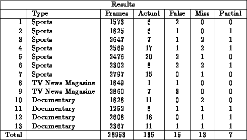
We ran experiments for the gradual transition detection procedure over
13 clips containing many types of gradual transitions such as dissolves, fades,
wipes, and other special effect edits. There were a total of 28953 frames
tested containing 135 gradual transitions. These clips contained a wide
variety of content including sporting events, documentary clips of wild-life
and natural habitats, and prime-time TV news magazines. Within the sports
clips, there were also many documentary-style features of athletes.
First, we generated the VideoTrail for each clip and split it into its
constituent stationary and transitional trails. We then ran the classification
algorithm on each trail, and compared the ranges of each transitional
trail with the motion ranges detected by the global motion detector. Using
a small tolerance (10 frames) at each end of the range,
we determined whether a transitional trail was due to motion or due to
a gradual transition edit. Using the ground truth of those clips,
we were able to identify the number of false detections and missed detections.
Apart from those two standard errors, we also computed partial range
matches where the ranges did not match within the prescribed tolerances.
The results of the experiments are summarized in Table 1.
Table 1: Results of the Gradual Transition Detection Experiments
Most cases of false detections were due to the inability of the motion
detector to detect a consistent motion pattern. Our performance is therefore
limited by factors such as the quality of motion estimation used during the
encoding of MPEG clip. A typical case leading to missed detections was when
an edit combined similar shots due to which the trail segmentation procedure
was unable to split the VideoTrail at the edit points. This is the case, for
example, when a transition occurs between shots from two cameras focused on
the same scene. Some missed detections were due to the fact that one or both
of the shots being combined with a special effect edit could be undergoing
motion as the edit occurs. In such cases, the motion detector misclassified
gradual transitions as motion transitions. Most partial detections resulted
from the same ambiguity.
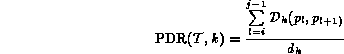
Tolerating the partial detections, the table shows that we obtained a recall
rate of 90.4% ( ), and a
precision of 89.1% ( ),
indicating that we were able to achieve good performance using this
technique. We are currently in the process of evaluating the performance of
our algorithm with respect to existing gradual transition detection algorithms,
and we hope to present the results of our comparison in the future.
In addition to the application to the gradual transition detection problem
explained earlier, there are other areas where the VideoTrails
representation is of primary interest.
Video sequences often contain different shots of the same content. This is
typically the case when a scene is shot with a small number of stationary
cameras focused on particular objects. We explained earlier that similar
frames in a video clip are transformed into points close together in the low
dimensional space. This is also true of frames taken from different shots of
the same content. Hence, two shots of the same content will yield clusters
that overlap to a significant degree in the VideoTrails
representation. These overlaps can easily be detected by comparing the
individual MBRs of stationary trails and testing for their overlaps.
A typical conversational scene between two
persons has three distinct camera angles, one for each person, and a third
for a medium shot capturing both persons. A VideoTrail representation
of these shots would contain three fairly large stationary trails
with transitions occurring frequently amongst them. On the other hand,
action sequences typically contain many transitional trails corresponding
to shots with high activity. There would be little inter-shot similarity
amongst the action shots. Earlier work on this problem can be found
in [17].
Judicious selection of key frames is important
in many applications, especially in extracting features for indexing video.
An ideal key frame for a shot should be representative of all the frames of a
shot. Applying simple heuristics like always choosing the first frame of a
shot might not be a good idea in certain cases. Instead, key frames can be
chosen from the clusters in the VideoTrail representation. For example,
the point closest to the center of the MBR of the cluster could be a better
representative. Another choice could be the point closest to the center of
mass or centroid of the cluster.
The key frame concept can also be extended in the following manner. We can use
the points chosen for key frames to represent the entire cluster, and if
we create directed edges between these key frame points, we can develop
a directed graph representation of the entire video clip which can be used
for performing analysis for extracting story units [17].
Certain types of video clips have a standard structure which can be
used to classify other videos having the same structure. For example,
a typical half-hour local news report has one or two standard shots
of news anchors interspersed with shots of on-location news clippings.
The weather and sports reports will have their own anchor person shots
occurring frequently mixed with sports sequences. Thus, the directed graph
of such a program will have a clique formed by a few prominent high degree
nodes corresponding to these shots of anchor persons. There will also be
many non-overlapping self loops leaving and returning to these anchor person
shots corresponding to news items. The weather and sports anchor shots
will have their own set of self loops. If the directed edges along these self
loops are collapsed to form a single self loop, distinct structure
can be identified. Using graph matching techniques, it is possible to
classify videos of other news programs having the same structure.
Figure 5 is an example of how a typical news structure looks
like.
Figure 5: Example of a news clip representation after directed edges
in a self loop to a clique are collapsed. The black dots represent news
anchor shots.
We have presented a technique which can be used to provide a compact representation of a video sequences structure. The technique reduces a sequence MPEG
encoded video frames to a trail of points in a low dimensional space. In
this space, we can cluster frames, analyze transitions between clusters and
compute properties of the resulting trail. By classifying portions of the
trail as either stationary or transitional, we are able to detect gradual
edits between shots. Furthermore, tracking the interaction of clusters over
time, we lay the groundwork for the complete analysis and representation of
the video's physical and semantic structure.
One primary observation of this work is that transitions
are indicated as much by consistency and differences between the
content of the surrounding shots as they are by characteristics of the
transitions themselves. By exploiting these consistencies through
clustering, we are able to analyize the higher level structure.
Our current work is concentrating on video classification and browsing.
Of the 64 DCT coefficients, the coefficient with zero
frequency in both dimensions is called the `DC coefficient', while the
remaining 63 are called the `AC coefficients'.
Y. Ariki and Y. Saito.
Extraction of TV news articles based on scene cut detection using
DCT clustering.
In Proc. of the IEEE International Conference on Image
Processing, volume 3, pages 847-850, 1996.
F. Arman, A. Hsu, and M.Y. Chiu.
Image processing on compressed data for large video databases.
In Proc. of the ACM Multimedia Conference, pages 267-272,
1993.
M. Cherfaoui and C. Bertin.
Two-stage strategy for indexing and presenting video.
In Proc. of the SPIE Conference on Storage and Retrieval for
Image and Video Databases II, volume 2185, pages 174-184, 1994.
C. Faloutsos and K. Lin.
FastMap: A fast algorithm for indexing, data-mining and
visualization of traditional and multimedia datasets.
In Proc. of the ACM SIGMOD Conference, pages 163-174, 1995.
C. Faloutsos, M. Ranganathan, and Y. Manolopoulos.
Fast subsequence matching in time-series databases.
In Proc. of the ACM SIGMOD Conference, pages 419-429, 1994.
P. Kelly, A. Gupta, and R. Jain.
Visual computing meets data modeling: Defining objects in
multi-camera video databases.
In Proc. of the SPIE Conference on Storage and Retrieval for
Still Image and Video Databases IV, volume 2670, pages 120-131, 1996.
V. Kobla, D. Doermann, and K. Lin.
Archiving, indexing, and retrieval of video in the compressed domain.
In Proc. of the SPIE Conference on Multimedia Storage and
Archiving Systems, volume 2916, pages 78-89, 1996.
V. Kobla, D. Doermann, K. Lin, and C. Faloutsos.
Feature normalization for video indexing and retrieval.
CfAR Technical Report CAR-TR-847 (CS-TR-3732), University
of Maryland, 1996.
V. Kobla, D. Doermann, K. Lin, and C. Faloutsos.
Compressed domain video indexing techniques using dct and motion
vector information in MPEG video.
In Proc. of the SPIE Conference on Storage and Retrieval for
Still Image and Video Databases V, volume 3022, pages 200-211, 1997.
V. Kobla, D. Doermann, and A. Rosenfeld.
Compressed domain video segmentation.
CfAR Technical Report CAR-TR-839 (CS-TR-3688), University
of Maryland, 1996.
J. Meng, Y. Juan, and S.F. Chang.
Scene change detection in a MPEG compressed video sequence.
In Proc. of the SPIE Conference on Digital Video Compression:
Algorithms and Technologies, volume 2419, pages 14-25, 1995.
B. Shahraray.
Scene change detection and content-based sampling of video.
In Proc. of the SPIE Conference on Digital Video Compression:
Algorithms and Technologies, volume 2419, pages 2-13, 1995.
B.L. Yeo and B. Liu.
On the extraction of DC sequence from MPEG compressed video.
In Proc. of the IEEE International Conference on Image
Processing, volume 2, pages 260-263, 1995.
B.L. Yeo and B. Liu.
Unified approach to temporal segmentation of motion JPEG and MPEG
video.
In Proc. of the International Conference on Multimedia Computing
and Systems, pages 2-13, 1995.
M. Yeung and B.L. Yeo.
Video content characterization and compaction for digital library
applications.
In Proc. of the SPIE Conference on Storage and Retrieval for
Still Image and Video Databases V, volume 3022, pages 45-58, 1997.
R. Zabih, J. Miller, and K. Mai.
Feature-based algorithm for detecting and classifying scene breaks.
In Proc. of the ACM Multimedia Conference, pages 189-200,
1995.
D. Zhong, H. Zhang, and S.F. Chang.
Clustering methods for video browsing and annotation.
In Proc. of the SPIE Conference on Storage and Retrieval for
Still Image and Video Databases IV, volume 2670, pages 239-246, 1996.
 of I frames, we can estimate
the DC coefficients of MBs of P and B frames with minimal computation
[15]. This results in a uniform representation of the spatial data of
all types of frames of an MPEG clip. We utilize the DC coefficients of the
luminance and chrominance components of an MPEG frame as features and the
Euclidean distance between the feature vectors to test for similarity between
frames. Using a technique called FastMap [5], we
perform dimensionality reduction to generate a low-dimensional vector for
each frame. Since the feature extraction has
been described in previous work[9, 10], we continue with a
description of the dimensionality reduction.
of I frames, we can estimate
the DC coefficients of MBs of P and B frames with minimal computation
[15]. This results in a uniform representation of the spatial data of
all types of frames of an MPEG clip. We utilize the DC coefficients of the
luminance and chrominance components of an MPEG frame as features and the
Euclidean distance between the feature vectors to test for similarity between
frames. Using a technique called FastMap [5], we
perform dimensionality reduction to generate a low-dimensional vector for
each frame. Since the feature extraction has
been described in previous work[9, 10], we continue with a
description of the dimensionality reduction.